UNDERSTANDING ALIASING AND SAMPLING USING PYTHON

~Bakyalakshmi

Sampling theorem:

fs≥2fm

A continuous time signal can be represented as samples and can be recovered back when sampling frequency f_sis greater than or equal to twice the highest frequency component of message signal.
If this condition does not satisfy, it leads to aliasing.
Aliasing is an effect that causes different signals to become indistinguishable when sampled.

Visualizing using python:

import matplotlib.pyplot as plt # to plot

import numpy as np

#numerical python to get array of float values and for sine operation

t = np.arange(0, 2e-3, 10e-6) # x axis time period

# sampling at fs =10kHz in time domain ts=1/fs (0.1ms)

ts = np.arange(0,2e-3,0.1e-3)

f = 1000 # message signal fm

b = np.sin(2*np.pi*f*t) #phase for sinewave

c = np.sin(2*np.pi*f*ts)

plt.plot(t,b,”g”) # plot of message signal (1kHz)

plt.plot(ts,c,”k*”) # plot of sampled message signal (1kHz)

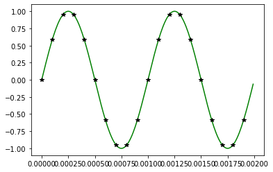
fs>=2fm: Input frequency= 1kHz sampling frequency = 10kHz

f=9000

b = -np.sin(2*np.pi*f*t)

c = -np.sin(2*np.pi*f*ts)

plt.plot(t,b) # plot of message signal (9kHz)

plt.plot(ts,c,’r+’) # plot of sampled message signal (9kHz)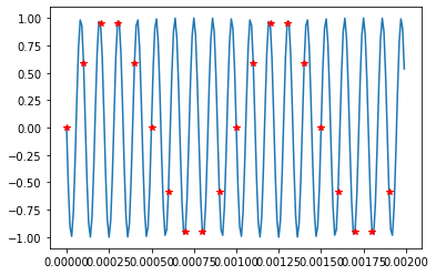

fs<2fm: Input frequency = 9kHz sampling frequency = 10kHz

Sampled output of 1kHz and 9kHz :

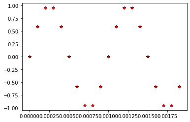
Aliasing of 1kHz and 9kHz